
Python Meets Policy: Understanding Catastrophic Health Spending in Malawi
A few years ago, I was just a young enthusiast; curious about data analysis, fascinated by numbers, and excited by the idea that data could tell real human stories. I never imagined that one day I would be standing before an academic panel, defending a full master’s thesis powered almost entirely by Python. My research, titled “Catastrophic Health Expenditures in Malawi: Distribution, Determinants, and Poverty Implications,” used the Integrated Household Survey (IHS5), a nationally representative dataset of 11,434 households. This wasn’t classroom data. It was huge, messy, complex, and a multidimensional survey data collected for national policy and economic planning. At first, I genuinely had no idea how I would manage it. But Python changed everything.
Motivation: What Was This Analysis Really About?
My study focused on health spending, specifically Catastrophic Health Expenditures (CHE).
Sounds dramatic, right? I thought so too the first time I heard it. But here’s the simple explanation:
Catastrophic health expenditure occurs when out-of-pocket health expenses become so high that they push a household into financial hardship; or even into poverty.
These costs include medication, transportation to hospitals, consultation fees, and any direct payments made for health care. When these expenses are large enough to destabilize a family’s finances, they’re considered catastrophic.
So, what exactly was I doing?
I wanted to identify what factors increase the likelihood that Malawians experience CHE, How widespread this financial hardship is, And just how deep the impact goes.
And yes, I found all of that.
Was This Research Even Necessary?
Absolutely! We live in a world that increasingly recognizes health as a fundamental human right. Everyone, regardless of geography or income, should have access to affordable, quality health services. This is the heartbeat of Sustainable Development Goal 3 (SDG 3) and the principle of Universal Health Coverage (UHC). Forget the jargon!. It simply means: Health for everyone. If people are being pushed into poverty because they sought healthcare, then we have a serious problem worth studying.
What Exactly Did I Set Out to Do?
I had three clear objectives:
- To estimate the incidence, intensity, and distribution of catastrophic health expenditures across households in Malawi.
- To assess the poverty impact of out-of-pocket health expenditures.
- To identify the determinants (the factors that increase or decrease the likelihood) of experiencing CHE.
Let Me Walk You Through My Analysis Stages?
My analysis unfolded in four major stages: Data Management & Pre-Processing; Descriptive Analysis; Econometric Modelling; and Interpretation, Discussion & Recommendations
1. Data Management & Pre-Processing
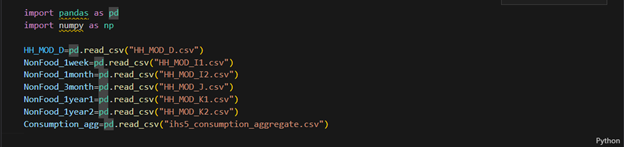
Importing Libraries and Datasets
Every analysis has to start somewhere. For me, it began in my VS Code Jupyter Notebook, where I first imported the essential libraries; pandas and numpy. With those in place, I loaded the CSV files containing the IHS5 survey datasets. This step simply brought all the raw data into Python, ready for the cleaning and transformation that would follow.
Making Sense of Strange Column Names
Look at what I saw when I opened the first dataframe, HH_MOD_D; a sea of cryptic codes that gave zero hints about what the columns actually meant. It was like trying to read a foreign language without a dictionary!

Well, at least I knew the dataset had health expenditure information What saved me? The questionnaire! I opened the survey tool to match each code to its meaning.
🌟 Fun Fact: SPSS Saved My Sanity: Honestly… lol, SPSS helped even more. I opened the SPSS file of the same dataset, and the variable labels popped up instantly, showing exactly what each column represented. That made everything so much easier. The questionnaire became Plan B. Moral: Even in a high-tech world, sometimes classic tools and simple solutions are the heroes; at least until you figure things out!!
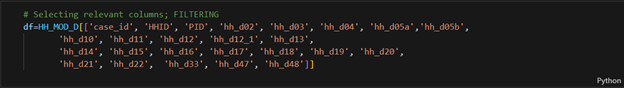
Selecting Relevant Columns (Filtering)
Using the SPSS labels, I filtered 25 health expenditure columns out of 60. No renaming yet; just keeping what mattered for calculating total out-of-pocket spending. The rest? Not useless, just not needed… yet.
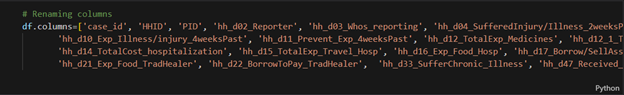
Renaming Columns
Next, I renamed the columns, still guided by SPSS. I created my own naming style; kept a hint of the original, but let’s be honest… lol, not exactly beautiful names. Well, obviously you are interested to decode the mystery behind these names… lol. Nothing mysterious anyway, just columns for expenditures associated with health, and of course I got you covered. Kindly checkout the column meanings in the code dictionary below. Only the relevant ones!
Calculating Totals for Each Expenditure Type
Ready for some code? This study was all about money, money, money. Some expenses were reported by multiple household members, so I used groupby() to sum each type per household.
🌟 Fun Fact: Early Aggregation Won
I did those calculations before handling missing values on purpose. Why? Aggregating similar expenditures early made everything else simpler. Who knew doing things “out of order” could be so smart!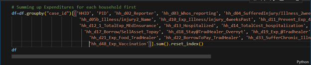
Missing Values
Good news! I found no missing values; which means every household spent something on health. Talk about universal participation!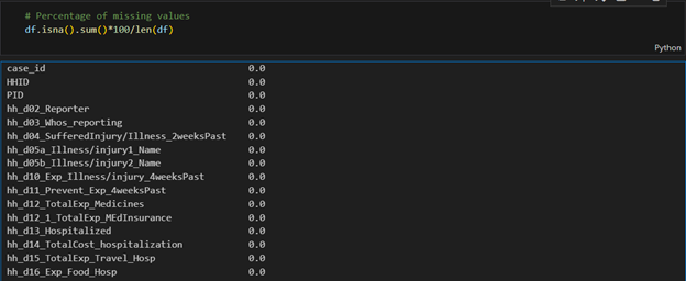
Creating Aggregate Columns and Standardizing Data
At this stage, I created new columns like Total Out-of-Pocket Expenditures, Total Household Expenditure, and Total Non-Food Expenditure; basically, turning the original dataset into one tailored for my analysis. The math? Just addition, nothing fancy.
Next came annualizing expenditures. Since the survey recorded spending over different periods; weekly, monthly, quarterly, yearly, I standardized everything to an annual measure by multiplying appropriately: weekly by 52, monthly by 12, and quarterly by 4.
Mapping symptoms to new symptom categories
Finally, I tackled the illnesses. Many had similar symptoms, so I grouped them into new categories and renamed some for clarity. Python’s map() function made this surprisingly easy.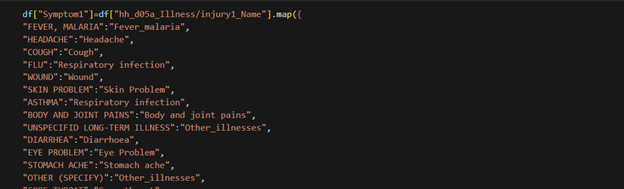
NOTE: I did a similar recategorization for several other variables e.g. health seeking behavior.
🌟 Fun Fact: The Great Variable Rebellion 😅
Did my initial variable mapping work? Nope. Some groups had just one observation! I had to recategorize and simplify; fewer categories, cleaner results.
Moral: Data sometimes has a mind of its own; you just have to dance with it, not against it.
Creating Wealth Quintiles
I categorized households into five wealth levels using Python’s qcut() function; Level 1 for the poorest, Level 5 for the richest. Each household was assigned a level based on its Total Asset value, which I had to calculate first.
Was this necessary? Absolutely! It makes targeting groups for policy analysis or interventions much easier, and a lot more meaningful.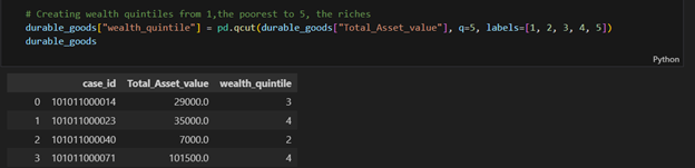
Multiple Dataframes and the Order of Operations
You might have noticed I’m not always using the usual df here. True! While I mostly refer to df for clarity, some operations were done in different dataframes; basically, I created smaller datasets relevant to each part of the analysis.
Fun fact: And a quick note: these data management steps weren’t done in the exact order I’ve described. In practice, I moved around as needed, though some steps naturally had to come before others.
2. Descriptive Analysis
This was another stage where Python truly became my partner. There were so many repetitive calculations that doing them by hand would have been exhausting. But with Python, I could write a simple for loop, run it, and let “Mr. Snake” deliver a basket of results while I took a breather.
Domain knowledge was key here. To answer my first two objectives, I needed to compute the incidence (prevalence) and intensity of Catastrophic Health Expenditures, as well as the same measures for poverty. My background in Development Economics and its toolbox of formulas came in handy, making the data speak clearly.
Objective 1: Estimating Catastrophic Health Expenditures
To measure how many households were pushed into financial hardship by health spending and how serious that hardship was, I used two common indicators. The first, CHE incidence (headcount), captures the prevalence of catastrophic health expenditures. The second, CHE Mean Positive Overshoot (MPO), measures their intensity.
To calculate CHE incidence, I applied a threshold: if a household’s out-of-pocket health spending exceeded 40% of its non-food expenditure, it counted as experiencing financial hardship. Simple, yet powerful, this approach turned raw spending data into meaningful insights about who was truly struggling.
Calculating Total Out-of-Pocket (OOP) Expenditure
How did I calculate a household’s total health spending? Simple; I just added the expenditure columns together. Sure, I might do it differently today, but that’s the beauty of coding: there’s always more than one way to get it done!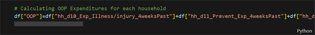
Calculating OOP Share
Was calculating total OOP enough for the CHE indicators? Not quite. I also computed OOP Share (OOPSHARE) by dividing each household’s total OOP by its Total Non-Food Expenditure; that column we created earlier during data management. Simple ratios, big insights!
Calculating CHE Headcount (Prevalence/Incidence)
First, I checked whether a household’s OOP Share exceeded the 40% threshold and created a new column for CHE status. Simple yes/no, but it revealed the prevalence of financial hardship:
df["CHE_40"]=np.where(df["OOPSHARE"]>0.4, 1, 0)
Then I calculated Che headcount/prevalence/incidence (H in this code) by
H= df["CHE_40"].mean()*100
Next came Mean Positive Overshoot (MPO), which measures the intensity of CHE among households exceeding the threshold. Firstly, I calculated how much each household went over 40%, the “CHE overshoot”, and stored it in a column called CHE_OVERSHOOT_40.
df["CHE_OVERSHOOT_40"]=df["OOPSHARE"]-0.4
Then I calculated MPO. Don’t be scared by the fancy name; it’s just the average overshoot, but only for households that exceeded the 40% threshold, not all households. Simple math, big insight!
MPO=df["CHE_OVERSHOOT_40"].sum()/len(df[df["CHE_40"] == 1])*100
A Quick Note on Thresholds
I repeated the same calculations, but this time the threshold was 10% of Total Health Expenditure instead of non-food expenditure. Same method, just a different benchmark—more ways to peek into financial hardship!
Analyzing Variations in CHE: Where Python Wins!
To see how financial hardship varied across groups; Urban vs. Rural, different wealth quintiles, and so on; I did a subgroup analysis. The calculations were the same as before, but repeated many times. That’s where Python’s for loops came to the rescue!
For example, a nested loop let me calculate CHE incidence at different thresholds for households grouped by various disease conditions; fast, accurate, and far less boring than doing it manually.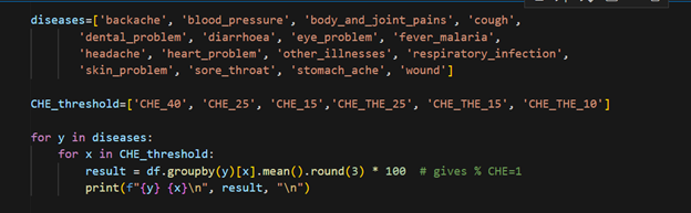
Objective 2: Assessing Poverty Due to Health Spending
Next up: poverty caused by out-of-pocket health expenses. After CHE, this part is a bit easier.
First, the Impoverishment Headcount; how many households were pushed below the poverty line because of health spending? I used a poverty line threshold: if a household’s per capita annual expenditure (calculated earlier) fell below this line, it was classified as poor.
This first step checks the poverty status of each household before paying for health; think of it as the “gross” view. Yes, I’m talking a lot… but hey, coding makes it way easier than it sounds!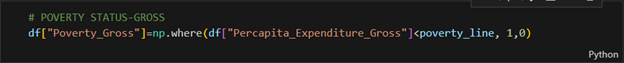
Poverty Status After Health Spending
The second step checks each household’s poverty status after out-of-pocket health payments; the “net” view. This shows exactly who got pushed below the poverty line because of health expenses.
Impoverished by Health Expenses
A household is considered impoverished if it was not poor before health spending (gross) but became poor after paying for health (net). I implemented this logic directly in Python to flag those households.
Finally, I just calculated the percentage of those that were impoverished; that is they were only poor after paying for health.
Impoverishment Gap
Next, I looked at the depth of impoverishment—how much deeper into poverty did health spending push already poor households? I calculated the poverty gap for each household before paying for health to set the baseline.
df["Poverty_Gap_Gross"] = np.maximum((poverty_line - df["Percapita_Expenditure_Gross"]) / poverty_line, 0)
Then i used this code to calculate the average poverty gap for each household before paying OOP.
average_poverty_gap_Gross = df["Poverty_Gap_Gross"].mean()*100).round(1)
Similary this piece of code below helped me calculate the poverty gap for each household after paying for health.
df["Poverty_Gap_Net"] = np.maximum((poverty_line - df["Percapita_Expenditure_Net"]) / poverty_line, 0)
Too much imformation here right? You’re not alone, but we’re anyway almost there.
Next, I calculated average poverty gap after paying for health.
average_poverty_gap_Net = (mergedAggregates["Poverty_Gap_Net"].mean()*100).round(1)
Finally, I calculated the change in poverty gap caused by health spending; the Impoverishment Gap. This shows exactly how much deeper households were pushed into poverty due to out-of-pocket health expenses.
Impoverishment_gap = average_poverty_gap_Net -average_poverty_gap_Gross
Well done!!!!!! 👏 Reaching this far, you’re already a health economist… a techy one at that!!
🌟 Fun Fact: I Thought Python Would Do It All Alone 😅
When I first opened the IHS5 dataset, I honestly thought Python would magically make sense of it all. Rows, columns, cryptic codes; my brain went on vacation. Little did I know, it wasn’t just Python that would carry me through; it was a mix of persistence, curiosity, and a few old-school tricks along the way.
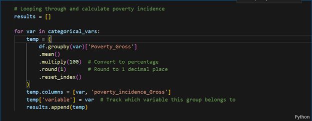
Analyzing Variations in Poverty Rates: Where Python Wins
To see how poverty rates varied across different groups, I needed to calculate them by category. Lots of repetition? Perfect job for a for loop! First, I defined the categorical variables I wanted to analyze, making it easy to run the calculations across all groups.
First, I defined the categorical variables I wanted to analyze:
categorical_vars=['region_name','reside_name','insurance_status', 'Chronic_illness_presence', 'hh_b03_Sex', 'wealth_quintile', 'very_young,<5 years', 'children, 6-14 years',
'youth, 15-24 years', 'adults, 25-54 years', 'middle_aged, 55-64 years',
'elderly, >65 years', 'sex_head', 'head_education', 'location',
'ageGroup', 'householdSizeGroup']
Then, I looped through this list to calculate the incidence of poverty for each category—fast, efficient, and way less boring than doing it manually.
3. The Regression Model: The Heart of the Study
The Regression Model: The Heart of the Study
After the descriptive phase, I built a binary logistic regression model to see which factors predicted the likelihood of catastrophic health spending. Python made it easy to fit the model and display results clearly. The output showed exactly which household characteristics increased or reduced the risk of catastrophic health expenditure.
Remember, I was investigating what drives households into financial hardship. Likely suspects included: age and gender of the household head, education level, household income, rural or urban location, number of illnesses, and type of health facility visited.
Of course, neither pandas nor numpy could handle regression estimates, so I brought in statsmodels to get the job done.
import statsmodels.formula.api as smf
Then I wrote a formula that puts together explanatory variables of the model
formula = """
CHE_40 ~ insurance_status + Chronic_illness_presence + C(wealth_quintile)
+ sex_head + C(ageGroup_head) + C(Education_head) + C(location)
+ C(householdSizeGroup) + C(region)
+ very_young_under5 + children_6_14_years + youth_15_24_years
+ adults_25_54_years + middle_aged_55_64_years + elderly_over65_years
+ C(backache) + C(blood_pressure) + C(body_and_joint_pains) + C(cough) + C(dental_problem)
+ C(diarrhoea) + C(eye_problem) + C(fever_malaria) + C(headache) + C(heart_problem)
+ C(other_illnesses) + C(respiratory_infection) + C(skin_problem) + C(sore_throat)
+ C(stomach_ache) + C(wound)
+ C(Did_nothing) + C(Government_facility) + C(Informal_commercial_sources)
+ C(Mission_CHAM_facility) + C(Private_facility) +C(Traditional_personal_remedies)
"""
Model Specification and Estimation
Next, I specified the logistic regression model using logit from statsmodels (smf), with my formula and data stored in df:
model = smf.logit(formula=formula, data=df)
Estimating model coefficients
Then I fitted the model to generate regression estimates, stored in a variable called results. To handle any potential heteroskedasticity in the residuals, I used robust standard errors (HC1). And just like that, my model was ready for interpretation!
result=model.fit(cov_type="HC1")
To check the output, I simply ran:
print(result.summary())
And voilà! Python delivered a neat table of regression estimates, ready for interpretation.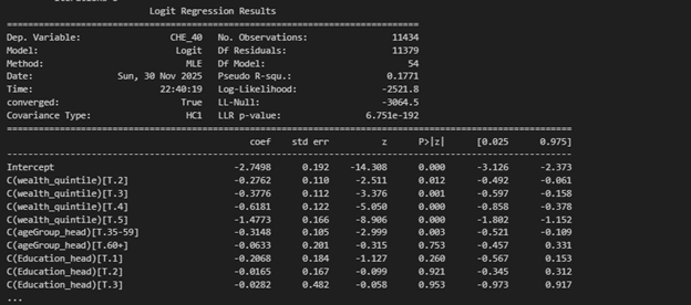
Converting Coefficients to Odds Ratios
The regression results shows log-odds coefficients, but I wanted odds ratios; much easier to interpret. First, I extracted the parameters and confidence intervals from the results output. Then, with a bit of Python magic, I converted both the coefficients and their CIs to odds ratios.
Extracting regression details
coef = result.params
conf = result.conf_int()
conf.columns = ["2.5%", "97.5%"] #Renaming confidence interval columns
Computing odds ratios and Confidence Intervals (CI)
OR = np.exp(coef)
CI_lower = np.exp(conf["2.5%"])
CI_upper = np.exp(conf["97.5%"])
- Interpretation, Discussion, Recommendations; Bringing the Results to Life
NOTE: The full analysis, with detailed results and regression models, will appear in a journal. For now, the story is clear: Python turned raw data into human stories.
After all the Python work, what did the numbers show? Simply put: health spending in Malawi is risky business. Rural households, female-headed households, and those with very young or elderly members were most vulnerable. Chronic illnesses added extra financial stress. Where households sought care mattered a lot.. Richer households were better protected, highlighting inequality in health spending. Out-of-pocket expenses didn’t just pinch; they pushed some households into poverty and deepened poverty for those already struggling.
The key takeaway? Sociodemographic factors, illness types, and health-seeking behavior all shape financial risk. Policies for financial risk protection are essential to prevent households from being pushed into hardship.
Lessons from the Journey & Final Thoughts
Data analysis isn’t just coding; it’s curiosity, persistence, and storytelling. Python was my toolkit; domain knowledge was my compass. Numbers don’t just sit in tables—they reveal real lives and struggles.
If you’re starting out: start small, be patient, stay curious, embrace errors, build consistently, and trust the process. One day, Python might quietly carry you from beginner to analyst… to researcher… to graduate. And your data story will be worth telling.
Coding Dictionary
- Selected Column names and their description
| Column name | Description |
| Case_id | Unique Household Identifier |
| HHID | Survey Solutions Unique HH Identifier |
| PID | Person ID on HH Roster |
| hh_d10_Exp_Illness/injury_4weeksPast | Amount spent for all illnesses and injuries, including for medicine, tests, consultation, & in-patient fees
|
| Hh_d11_Prevent_Exp_4weeksPast | Amount spent on medical care not related to an illness - preventative health care, pre-natal visits, check-ups, etc.
|
| hh_d12_1_TotalExp_MEdInsurance | Amount spent on medical insurance
|
| hh_d12_TotalExp_Medicines | Amount spent on non-prescription medicines and other medical products - Panadol, LA, cough syrup, contraceptives, etc
|
| Hh_d14_TotalCost_hospitalization | Total cost of your hospitalization(s) or overnight stay(s) in a medical facility
|
| Hh_d15_TotalExp_Travel_Hosp | Amount spent on travel to medical facility for overnight stay(s)
|
| Hh_d16_Exp_Food_Hosp | Amount spent on food during overnight stay(s) at medical facility |
| hh_d21_Exp_Food_TraHealer | Amount spent on food during overnight stay(s) at the traditional healer's or faith healer's dwelling |
| hh_d48_Exp_Vaccination | Amount spent on vaccination
|
- Python Functions, Libraries, and Their Use in the MSc Thesis Analysis
| Function/Method | Library | General Python Programming Use | Specific Use in MSc Thesis Analysis |
| I. Data Management & Pre-Processing | |||
| pd.read_csv() | pandas | Imports data from a CSV file into a DataFrame. | To import the raw IHS5 survey data files (e.g., 'HH\_MOD\_D.csv') into Python DataFrames. |
| .columns | pandas | An attribute to retrieve or set the list of column labels in a DataFrame. | To view the cryptic, raw column names of the loaded DataFrame. |
| df[...] | pandas | Used for column selection, either to retrieve columns for filtering or to create a new subset DataFrame. | Used for Selecting Relevant Columns (filtering) by specifying a list of 25 necessary health expenditure columns. |
| df.columns = [...] | pandas | Used to rename all columns at once by assigning a new list of descriptive string names. | To rename the filtered columns to more descriptive names, guided by the SPSS labels. |
| .groupby() | pandas | A crucial step for aggregation; it groups rows based on unique values in specified columns before applying a calculation. | Used to group data by case_id to Sum Up Expenditures for each household. |
| .sum() | pandas | Calculates the sum of values for the selected data. When applied with .isna(), it counts missing values. | Used with .groupby() to calculate the total for each expenditure type , and with .isna() to check for missing values. |
| .reset_index() | pandas | Converts the grouped column back into a regular column, resetting the index to be numeric. | Used after .groupby().sum() to make the resulting aggregated DataFrame cleaner. |
| .isna() | pandas | A method to identify Missing Values (NaNs) in the DataFrame. | Used to check for missing values, which were fortunately not found in this dataset. |
| .map() | pandas | A Series method used for substituting each value in a Series with another value, often using a dictionary (key-value mapping). | To Recategorize various illnesses/symptoms (e.g., 'FEVER, MALARIA') into new, simplified categories. |
| pd.qcut() | pandas | Discretizes a continuous variable into q equal-sized bins based on sample quantiles. | To create the five Wealth Quintiles (Level 1 to 5) based on each household's Total_Asset_value. |
| II. Descriptive Analysis | |||
| + (Addition) | Python/NumPy | The standard arithmetic operator for summation. | Used to calculate Total Out-of-Pocket (OOP) Expenditures by adding the expenditure columns together. |
| / (Division) | Python/NumPy | The standard arithmetic operator for division. | Used to compute the OOP Share (OOPSHARE) by dividing total OOP by Total Non-Food Expenditure. |
| np.where() | numpy | Returns elements chosen from two arrays based on a condition, essentially an "if-then-else" logic for arrays. | Core Logic Function used to create all binary status variables (1 or 0), including CHE_40, Poverty_Gross, Poverty_Net, and Impoverished. |
| len() | Python | Returns the number of items in an object (e.g., the number of elements in a list, or rows in a filtered DataFrame). | Used in the denominator of the MPO calculation to get the count of households experiencing CHE. |
| .mean() | pandas | Calculates the average of a Series. When applied to a binary column, it calculates the prevalence/proportion. | Used to calculate Incidence (Headcount) measures for CHE , Impoverishment , and Poverty , and also average poverty gaps. |
| .round(3) | pandas | Rounds the values in a Series or DataFrame to a specified number of decimal places. | Used within the for loop to format the percentage results for CHE incidence. |
| for loop | Python | A control flow statement that executes a block of code repeatedly over a sequence. | Used to automate repetitive Subgroup Analysis for both CHE and poverty incidence calculations across multiple categorical variables. |
| np.maximum() | numpy | Computes the element-wise maximum of two arrays, useful for clipping values at zero. | Used to calculate the Poverty Gap (Gross and Net) by ensuring the gap value is never negative (minimum is 0). |
| III. Econometric Modelling | |||
| smf.logit() | statsmodels | Specifies and sets up a Generalized Linear Model (GLM) for a logit link function, which is the standard method for Binary Logistic Regression. | Used to specify the Binary Logistic Regression Model predicting the likelihood of CHE_40. |
| model.fit() | statsmodels | The method used to Estimate the Model Coefficients by fitting the specified model to the data. | Used to fit the logistic model and applies the cov_type="HC1" parameter to use Robust Standard Errors. |
| result.summary() | statsmodels | Displays the standard output table for the fitted model, containing all regression statistics. | Used with print() to display the final Regression Output Table. |
| result.params | statsmodels | An attribute to Extract the Estimated Coefficients (log-odds) from the fitted model results. | Used to isolate the coefficients for converting them into Odds Ratios. |
| result.conf_int() | statsmodels | A method to Extract the Confidence Intervals (CIs) for the log-odds coefficients. | Used to isolate the CIs for converting them into Odds Ratio CIs. |
| np.exp() | numpy | Calculates the exponential of all elements in the input array. | To Convert Log-Odds Coefficients to Odds Ratios (ORs) and their corresponding confidence intervals. |