
A vector is a 1D array of values

We use the notation 𝑥𝑖 to denote the ith entry of x
Matrices
A matrix is a 2D array of values

We use 𝐴𝑖𝑗 to denote the entry in row 𝑖 and column 𝑗
Matrices and linear algebra
Matrices are:
Understanding both these perspectives is critical for virtually all data science analysis algorithms.
Matrices as tabular data
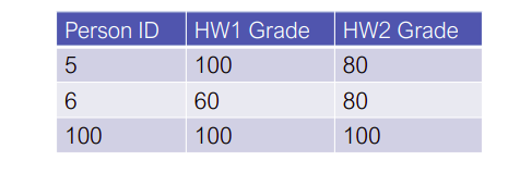
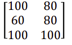
Ignoring the primary key column (this is not really a numeric feature, so makes less sense to store as a real-valued number), we could represent the data in the table via the matrix
Row and column ordering
Matrices can be laid out in memory by row or by column
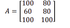
Row major ordering: 100, 80, 60, 80, 100, 100
Column major ordering: 100, 60, 100, 80, 80, 100
Row major ordering is default for C 2D arrays (and default for Numpy), column major is default for FORTRAN (since a lot of numerical methods are written in FORTRAN, also the standard for most numerical code)
Higher dimensional matrices
“Higher dimensional matrices” are called tensors
Systems of linear equations
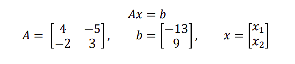
Consider two linear equations, two unknowns.
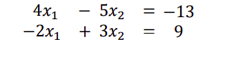
Matrices and vectors also provide a way to express and analyze systems of linear equations
We can write this using matrix notation as
Linear algebra computations underlie virtually all machine learning and statistical algorithms. There have been massive efforts to write extremely fast linear algebra code.
Numpy
In Python, the standard library for matrices, vectors, and linear algebra is Numpy. Numpy provides both a framework for storing tabular data as multidimensional arrays and linear algebra routines.
Important note: numpy ndarrays are multi-dimensional arrays, not matrices and vectors (there are just routines that support them acting like matrices or vectors).
Anaconda typically uses a reasonably optimized version of Numpy that uses one of these libraries on the back end
To check to see if Numpy is using specialized libraries, use the command:
import numpy as np
np.__config__.show()
Creating Numpy arrays
The ndarray is the basic data type in Numpy
b = np.array([-13,9]) # 1D array construction
A = np.array([[4,-5], [-2,3]]) # 2D array contruction
print(b, "\n")
print(A)
creating arrays/matrices of all zeros, all ones, or of random numbers (in this case, the np.randon.randn create a matrix with standard random normal entries, while np.random.rand creates uniform random entries).
print(np.ones(4), "\n") # 1D array of ones
print(np.zeros(4), "\n") # 1D array of zeros
print(np.random.randn(4)) # 1D array of random normal numbersprint(np.ones((3,4)), "\n") # 2D array of ones
print(np.zeros((3,4)), "\n") # 2D array of zeros
print(np.random.randn(3,4)) # 2D array of random normal numbers
Creating indentity matrix using the np.eye() command, and a diagonal matrix with the np.diag() command.
print(np.eye(3),"\n") # create array for 3x3 identity matrix
print(np.diag(np.random.randn(3)),"\n") # create diagonal array
Indexing into Numpy arrays
Using single indices and using slices, with the additional consideration that using the : character will select the entire span along that dimension.
A[0,0] # select single entry
A[0,:] # select entire column
A[0:3,1] # slice indexing # integer indexing
idx_int = np.array([0,1,2])
A[idx_int,3] # boolean indexing
idx_bool = np.array([True, True, True, False, False])
A[idx_bool,3]# fancy indexing on two dimensions
idx_bool2 = np.array([True, False, True, True])
A[idx_bool, idx_bool2] # not what you want
A[idx_bool,:][:,idx_bool2] # what you want
Basic operations on arrays
Arrays can be added/subtracted, multiply/divided, and transposed, but these are not the same as matrix operations
A = np.random.randn(5,4)
B = np.random.randn(5,4)
x = np.random.randn(4)
y = np.random.randn(5) A+B # matrix addition
A-B # matrix subtraction A*B # ELEMENTWISE multiplication
A/B # ELEMENTWISE division
A*x # multiply columns by x
A*y[:,None] # multiply rows by y (look this one up) A.T # transpose (just changes row/column ordering)
x.T # does nothing (can't transpose 1D array)
Basic matrix operations
Matrix multiplication done using the .dot() function or @ operator, special meaning for multiplying 1D-1D, 1D-2D, 2D-1D, 2D-2D arrays.
A = np.random.randn(5,4)
C = np.random.randn(4,3)
x = np.random.randn(4)
y = np.random.randn(5)
z = np.random.randn(4) A @ C # matrix-matrix multiply (returns 2D array)
A @ x # matrix-vector multiply (returns 1D array)
x @ z # inner product (scalar) A.T @ y # matrix-vector multiply
y.T @ A # same as above
y @ A # same as above #A @ y # would throw error
Solving linear systems
Methods for inverting a matrix, solving linear systems
b = np.array([-13,9])
A = np.array([[4,-5], [-2,3]]) np.linalg.inv(A) # explicitly form inverse
np.linalg.solve(A, b) # A^(-1)*b, more efficient and numerically stable
Important, always prefer to solve a linear system over directly forming the inverse and multiplying (more stable and cheaper computationally). Solution methods use a factorization (e.g., LU factorization), which is cheaper than forming inverse. Where L is a lower triangular matrix (all entries above the diagonal are zero), and U is an upper triangular matrix (all entries below the diagonal are zero).
Sparse matrices
Many matrices are sparse (contain mostly zero entries, with only a few non-zero entries)
Examples: matrices formed by real-world graphs, document-word count matrices (more on both of these later)
Storing all these zeros in a standard matrix format can be a huge waste of computation and memory. Sparse matrix libraries provide an efficient means for handling these sparse matrices, storing and operating only on non-zero entries.
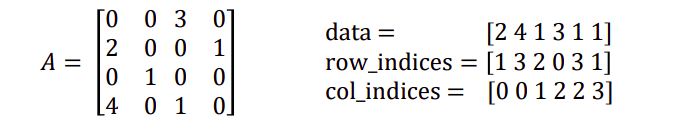
There are several different ways of storing sparse matrices, each optimized for different operations:
Coordinate (COO) format: store each entry as a tuple (row_index, col_index, value)
Compressed sparse column (CSC) format: Faster for matrix multiplication, easier to access individual columns but very bad for modifying a matrix, to add one entry need to shift all data.

Sparse matrix libraries
Need specialized libraries for handling matrix operations (multiplication/solving equations) for sparse matrices
General rule of thumb (very adhoc): if your data is 80% sparse or more, it’s probably worthwhile to use sparse matrices for multiplication, if it’s 95% sparse or more, probably worthwhile for solving linear systems)
The scipy.sparse module provides routines for constructing sparse matrices in different formats, converting between them, and matrix operations
import scipy.sparse as sp
A = sp.coo_matrix((data, (row_idx, col_idx)), size)
B = A.tocsc()
C = A.todense()