
A large amount of data in many real-world data sets comes in the form of free text (user comments, but also any “unstructured” field)
(Computational) natural language processing: write computer programs that can understand natural language
The goal here is using free text in data science is to extract some meaningful information from the text, without any deep understanding of its meaning. The reason for this is simple: extracting deep understanding from text is hard.
Understanding language is hard
Multiple potential parse trees:
“While typing at the office, I ran into some bugs. How it made me get home, I don’t know.” — Susan David
Winograd schemas:
“The city council members refused the demonstrators a permit because they [feared/advocated] violence.”
Basic point: We use an incredible amount of context to understand what natural language sentences mean
But is it always hard?
Two reviews for a movie
Which one is positive?
We can often very easily tell the “overall gist” of natural language text without understanding the sentences at all
In many data science problems, we don’t need to truly understand the text in order to accomplish our ultimate goals (e.g., use the text in forming another prediction)
We will discuss two simple but very useful techniques that can be used to infer some meaning from text without deep understanding
Note: These methods are no longer sufficient for text processing in data science, due to advent of deep-learning-based text models
Some key ideas that are also important to understand deep learning approaches to text/language
Terminology: Before we begin, a quick note on terminology. In these notes “document” will mean an individual group of free text data (this could be an actual document or a text field in a database). “Words” or “terms” refer to individual tokens separated by whitespace, and additionally also refers to punctuation (so we will often separate punctuation explicitly from the surrounding words. “Corpus” refers to a collection of documents, “vocabulary” or “dictionary” is the set of possible words in a language or just the set of unique terms in a corpus.
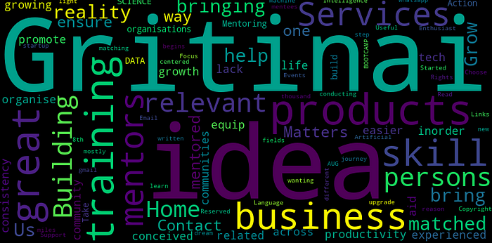
Also known as the word cloud view of documents. Each document a vector of word frequencies, also order of words is irrelevant, only matters how often words occur.
!pip install wordcloudimport wordcloudfrom bs4 import BeautifulSoup
import requests
import reresponse = requests.get("http://www.gritinai.com")
root = BeautifulSoup(response.content, "html.parser")
from wordcloud import WordCloud
wc = WordCloud(width=800,height=400).generate(re.sub(r"\s+"," ", root.text))
wc.to_image()
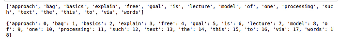
Bag of words example
documents = ["the goal of this lecture is to explain the basics of free text processing",
"the bag of words model is one such approach",
"text processing via bag of words"]document_words = [doc.split() for doc in documents]
vocab = sorted(set(sum(document_words, [])))
vocab_dict = {k:i for i,k in enumerate(vocab)}
print(vocab, "\n")
print(vocab_dict, "\n")
Now let’s construct a matrix that contains word counts (term frequencies) for all the documents. We’ll also refer to the term frequency of the jth word in the ith library as tf i,j.
import numpy as np
X_tf = np.zeros((len(documents), len(vocab)), dtype=int)
for i,doc in enumerate(document_words):
for word in doc:
X_tf[i, vocab_dict[word]] += 1
print(X_tf)
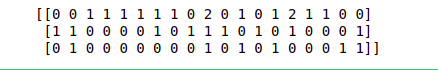
Each of the rows in this matrix corresponds to one of the three documents above, and each column corresponds to one of the 19 words.
Term frequency
“Term frequency” just refers to the counts of each word in a document
Denoted tf 𝑖,𝑗 = frequency of word 𝑗 in document 𝑖 (sometimes indices are reversed, we use these for consistency with matrix above)
Often this just means the raw count, but there are also other possibilities
Term frequencies tend to be “overloaded” with very common words (“the”, “is”, “of”, etc). Note: really common words, called “stop words,” may even be removed.
idf𝑗 = log(# documents / # documents with word 𝑗)
TFIDF
Term frequency inverse document frequency = tf𝑖,𝑗 × idf
Discouting words that occur very frequently, and increasing the weight of less frequent terms. This seems to work much better than using raw scores
Cosine similarity
One of the more common questions to address is to compute similarity between multiple documents in the corpus. The common metric for doing so is to compute the cosine similarity between two different documents. This is simply a normalize inner product between the vectors describing each documents.
Equivalent to the (1 minus) the squared distance between the two normalized document vectors.
The cosine similarity is a number between zero (meaning the two documents share no terms in common) and one (meaning the two documents have the exact same term frequency or TFIDF representation).
Term frequencies as vectors
Word embeddings and word2vec
One of the downsides to term frequency models (even as far as bag-of-words representations are concerned), is there is no notion of similarity between words. But in reality, we do associate some notion of similarity between different words. For example, consider the following corpus.
documents = [
"pittsburgh has some excellent new restaurants",
"boston is a city with great cuisine",
"postgresql is a relational database management system"
]
To get started with word embeddings, we’ll note that words in the term frequency model can also be considered as being represented by vectors; in particular, any word is represented by a “one-hot” vector that has a zero in all the coordinates except a one in the coordinate specified by the word. For example, let’s form the vocabulary for the corpus above.
document_words = [doc.split() for doc in documents]
vocab = sorted(set(sum(document_words, [])))
vocab_dict = {k:i for i,k in enumerate(vocab)}
print(vocab_dict, "\n")

e_pittsburgh = np.zeros(len(vocab))
e_pittsburgh[vocab_dict["pittsburgh"]] = 1.0
print(e_pittsburgh)
output
[ 0. 0. 0. 0. 0. 0. 0. 0. 0. 0. 0. 1. 0. 0. 0. 0. 0. 0.]
The (squared) distance between two words is either two (if the words are different) or zero (if the words are the same). Despite the fact that we think of “pittsburgh” and “boston” as being “closer” to each other than to “database”, our term frequency model doesn’t capture this at all.
Word embeddings : Like the one-hot encoding of words, a word embedding is a vector representation of words, in some space R^k.
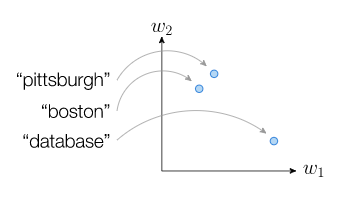
As seen in the figure, “similar” words are mapped to points close together (by Euclidean distance), whereas dissimilar words will be further away.
Word2vec : We haven’t talked about machine learning to properly cover this word2vec algorithm. The basic idea of word2vec is that, given a large body of text, we want to train an algorithm that can “predict” the context around a word. The idea here is that we try to slightly bump up the probability of the surround words, and lower the probability of other words.
While the bag of words model is surprisingly effective, it is clearly throwing away a lot of information about the text
The terms “boring movie and not great” is not the same in a movie review as “great movie and not boring”, but they have the exact same bag of words representations
To move beyond this, we would like to build a more accurate model of how words really relate to each other: language model
Probabilistic language models
A probabilistic language model attempts to to predict the probablity of each word in the document, given all the words that proceeded it
P(wordi|word1,…,word i−1)
E.g., you probably have a pretty good sense of what the next word should be: • “Data science is the study and practice of how we can extract insight and knowledge from large amounts of”
𝑃 word𝑖 = “data” word1, … , word𝑖−1) = ?
𝑃 word𝑖 = “pizza” word1, … , word𝑖−1) = ?
Of course, note that this also requires some information about language, to understand that “data” makes more sense given that the sentence is talking about data science.
We make simplifying assumptions to build approximate tractable models because building a language model that captures the true probabilities of natural language is still a distant goal.
N-gram model: the probability of a word depends only on the 𝑛 − 1 words preceding it
𝑃 word𝑖 |word1, … , word𝑖−1) ≈ 𝑃(word𝑖 |word𝑖−𝑛+1, … , word𝑖−1)
Laplace smoothing
Estimating language models with raw counts tends to estimate a lot of zero probabilities (especially if estimating the probability of some new text that was not used to build the model)
How do we pick 𝑛?
Hyperparameter
Lower 𝑛: less context, but more samples of each possible 𝑛-gram
Higher 𝑛: more context, but less samples
“Correct” choice is to use some measure of held-out cross-validation
In practice: use 𝑛 = 3 for large datasets (i.e., triplets) , 𝑛 = 2 for small ones
More on this to be explained later on!!